This instrument determines the Q (quality factor) of a resonant circuit, crystal, or resonator by measuring its series resistance at the resonance frequency. The Q is linked to the series resistance by two simple equations (RS is the series resistance, L and C the reactive elements and FR their resonance frequency):
This Q-meter is unusual on more than one count: it is capable of displaying directly the value of the series resistance, and is based on a series-tuned oscillator. The advantages associated with this type of oscillator have been described in another design idea [1].
Here the series-tuned topology shines because it introduces no damping of its own at the common node between L and C, and because the tank’s series resistance is accurately cancelled by a calibrated negative resistance. This negative resistance is therefore an accurate image of the resonant circuit’s losses, and nothing else.
Circuit description
The circuit is based on the cross-quad topology [2]: Q1 to Q4 form the quadruplet, and the circuit normally synthesizes a zero resistance between the emitters of Q3 and Q4, by cancelling parasitic parameters (Figure 1).
 |
|
| Figure 1. | |
Here, to use the circuit as an oscillator, some modifications have been made: the Zeners D1 to D4 ensure the transistors have enough C-E dynamic to “breathe” properly, and an adjustable positive feedback is introduced via pot P1 (yes, positive feedback is introduced from the collector of Q2 to its base; that’s how things work in the strange and inverted world of the cross-quad).
With this modification, the resistance between the wiper of P1 and ground appears with an opposite sign between the emitters of Q3 and Q4. When the magnitude of this resistance equals that of the tank circuit, the circuit starts to oscillate. The current in the other arm of the quad is intercepted by R1, and results in a voltage appearing on the diode detector D6/D7, and the output J1. D7 is a peak detector compensated by D6. When a signal is detected, it increases the voltage on the (–) input of U1b, and pulls the output down, lighting D8.
The cross-quad is biased by two current sources, Q5 and Q6, delivering precisely 5 mA thanks to U1a. This bias current also flows through P1, and generates a voltage drop equal to the setting of the potentiometer times 5 mA.
This voltage is divided by five by R15/R16, and sent to a millivoltmeter; the value displayed in mV now reflects exactly the potentiometer’s value in ohms. Thanks to this trick, the actual value can be displayed accurately, without having to resort to approximate scales or further calculations. The resonant frequency can be measured by connecting a frequency meter to J1.
The ×1/×10 switch can reduce the potentiometer’s apparent value by paralleling R8, bringing the full scale value to 22 Ω instead of 220 Ω. Because C7 blocks the DC, the displayed value is unaffected and retains its full resolution.
The role of many components has remained unexplained so far: L1 to L3, R2 to R7, C2, C4. They all contribute to the stability of the circuit, and suppress unwanted oscillations. Without them, the circuit could oscillate at UHF frequencies; the few centimetres of the test terminals form an open transmission line having resonant frequencies of its own, and since it has a very high Q, it would invariably dominate.
The additional components constrain the frequency range: here, the maximum usable frequency is about 100 MHz (to keep an acceptable accuracy). It is a trade-off between performance and usability. L1 to L3 are ferrite beads of ~80 nH (50 Ω). Needless to say that careful layout techniques are a must for a stable, proper operation.
Adjustments
In the absence of oscillation, TR2 has to be adjusted to keep the LED D8 just off, so that it lights as soon as an oscillation is present.
To adjust TR1, use a high quality tuned circuit in the 1 to 10 MHz range (polystyrene or silver mica capacitor, low loss inductor). Preset TR1 to read 0.5 V between its wiper and –12 V. Measure the resonant circuit on the 22 Ω (×1) range and note the value. Add a non-inductive 10 Ω precision resistor in series with the LC. Adjust P1 to the new value, and adjust TR1 to read 10 Ω + the initially measured value. Go through the procedure again: it normally converges very quickly, and one or two passes should be sufficient. Check that the indications remain consistent in the ×10 range.
Practical tips
With some types of components, ambiguities can sometimes appear: this is the case for low-frequency circuits and some types of resonators.
At low frequencies, the components are physically large, and the inductor has a significant parallel capacitance. The wiring and this capacitance thus form a “phantom” resonant circuit of a much higher frequency. It also has a higher Q than the “regular” circuit, because low-frequency inductors have a high ESR. All of this means that the tester will find the VHF resonance first; that is not a malfunction of the circuit, it is perfectly normal.
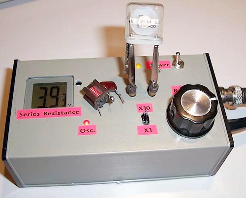
To force the circuit to operate at low frequencies only, the solution is to “kill” the HF response by including large ferrite beads in the circuit. The photograph (Figure 2) shows a practical way of implementing it: the test terminals are screw terminals directly attached to the PCB. For VHF operation, they can be used directly, but for general-purpose use, they are extended with alligator clips which are more convenient, and a large ferrite bead (1 µH/600 Ω) is added in series with each connection. This effectively forces the circuit to operate at frequencies <10 MHz.
 |
| Figure 2. |
The same type of problem can appear with mechanical resonators: the motional parameters are shunted by the physical capacitance, and this capacitance can resonate with the connection length. That is particularly true for ceramic resonators, having a much larger capacitance than crystals. The remedy is the same as above: add extra HF damping with beads, or an inductor shunted by a resistor.
Crystals present a problem of their own. They have a very large Q, and as a result, a large time-constant. This tester cancels the residual losses, thus increasing the apparent Q and the time-constant to near infinity! With a correct setting of P1, the build-up of oscillations can take up to a minute. This makes the adjustment near impossible – even if you turn P1 very slowly, by the time the LED lights, you will have overshot the right value by a large amount.
In this case, the simplest solution is to connect an oscilloscope to J1, and manually act as a “human AGC” by looking at the amplitude: the phenomena are so slow that it is easy to do. The oscillator behaves like a perfect integrator.
Other applications
Because of its inherent cancellation of parasitic parameters, this oscillator topology offers an outstanding stability, which can be used in other applications – proximity detectors for example – inductive if the coil is the sense element, or capacitive if the common node between the L and the C is the input.
It also finds the exact natural (series) resonance of a crystal very accurately, regardless of parasitic elements like shunt capacitance.
