This project will explain how to develop a system to measure magnetic field emissions at frequencies up to 150 kHz from high-current power cables without cutting or disturbing the cable.
Magnetic fields are present almost everywhere. However, convenient means of assessing the magnetic field strength over wide ranges of strength and frequency (20 Hz to 150 kHz) are not widely available. Despite the limitations, there are still many reasons why you may need these measurements. One example is tracking down the interference from an unshielded or poorly-shielded cable.
In this project, we will develop a method to evaluate magnetic field emissions at frequencies up to 150 kHz from high-current power cables without cutting or disturbing the cable.
To begin, we will need two simple analog instruments:
- A hand-held magnetic field meter with a field sensor probe
- A calibration reference verifier source capable of producing a magnetic field strength of up to 1000 A/m (amps per meter) or 1.26 mT
Generally, high-accuracy measurements are unlikely to be practicable or useful. This is because many magnetic field strengths, particularly at high frequencies, can vary considerably even over short periods and distances. In addition, it's important to note that the verifier overcomes a requirement for the instrument to have high intrinsic accuracy, but its stability is normally more than adequate.
A hand-held unit for measuring magnetic field strength
Let's dive into the development and components of the hand-held magnetic field strength unit. To begin with, let's look at a block diagram of the meter and verifier shown in Figure 1.
 |
|
| Figure 1. | Block diagram of the magnetic field meter and verifier. |
Note that the meter is powered by a single 9 V battery. From here, we'll break down the different necessary components.
Magnetic field probe and preamp
The probe consists of a 1.6 μH inductor that is 8 mm long and 7.5 mm in diameter. It is wound on an insulating former and has about 22 turns. An electrostatic shield (a single overlapped, insulated turn of copper foil) is provided. Regarding frequency response, the inductance value is not critical, but the physical dimensions affect the sensitivity. The probe is connected to a coaxial cable with the electrostatic shield connected to the cable shield.
The probe is directional, and normally it is placed with its axis vertical (assuming a horizontal cable) and senses the vertical component of the magnetic field. Still, the user can set it horizontally to measure the horizontal component.
Overall, the total field strength at a point is the square root of the sum of the squares of the vertical field, HV, and the two components of the horizontal field, HX and HY.
The schematic of the probe and preamp is shown in Figure 2.
 |
|
| Figure 2. | Probe and preamp schematic. |
The preamp is physically integrated with the main amplifier and shares a common ground. The output, X, from the preamp connects to the input, X, of the main amplifier schematic shown below in Figure 3.
 |
|
| Figure 3. | Main amplifier schematic. |
The preamp consists of a transconductance amplifier with a very low input impedance. This technique produces a flat frequency response from a mutual-inductance source. However, it can be impractical to obtain a low enough input impedance compared with the reactance of 1.6 μH at 20 Hz. One way to overcome this is to increase the inductance by a series 1 mH toroidal inductor insensitive to external magnetic fields. The resistance of the coil and the added 15 Ω resistor is compensated by including a capacitor in series with the 1 kΩ feedback resistor.
This inductor consists of about 20 turns on a ferrite toroid, 9.6 mm outside diameter, 4.7 mm inside diameter, and 3.2 mm thick. The Digi-Key part number of the toroid is 240-2522-ND. Commercially available 1 mH inductors are physically large parts designed to carry large currents and are unsuitable here.
Main amplifier
The amplifier has only a small gain and includes two filters. When driving a high-impedance load, the probe, preamp, and main amplifier provide a sensitivity of 1 mV for 1 A/m field strength at the probe. The SI unit A/m (amps per meter) is a ‘small’ unit, as opposed to the farad, for example, which is a ‘big’ unit, so we normally use parts whose capacitance is a very small fraction of a farad. How small? Well, 1 A/m produces a flux density of 1.26 μT (microtesla) in the air or a vacuum, whereas the magnet in an earbud produces around 1 T.
Previously in Figure 3, we showed the schematic for the main amplifier. In it, the first stage is a 3rd-order low-pass filter to eliminate noise above about 200 kHz.
The low-pass filter is followed by a 3rd-order high-pass filter, whose –3 dB frequency can be switched between 8 Hz and 800 Hz using switches S1a, S1b, and S1c. The switches can be implemented using a single 3-pole 2-way (or on-off) switch.
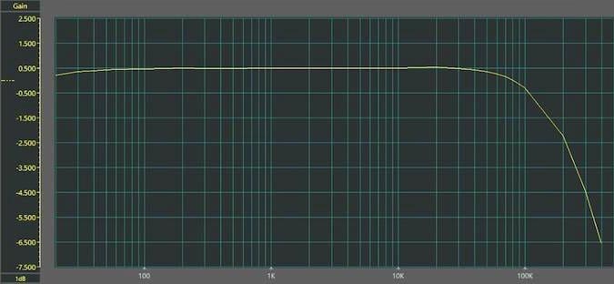
In Figure 3, the switches in the second stage are shown configured to produce an –3 dB frequency of 8 Hz from the second stage filter. This 8 Hz response is best for attenuating flicker noise in this wideband response mode. In this configuration, the full main amplifier provides a broadband output with a substantially flat response from below 20 Hz to 100 kHz and a limited fall up to 150 kHz, as shown in Figure 4. Because of the effect of other coupling capacitors (C2, C7, C11, C18), the –3 dB frequency of the full main amplifier response is 11 Hz.
 |
|
| Figure 4. | Main amplifier frequency response showing the 3rd-order low-pass filter configured for an 8 Hz response. |
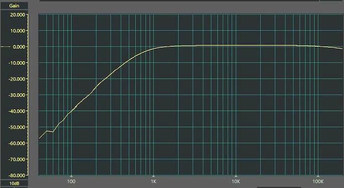
For the 800 Hz high-pass response, 1.5 kΩ resistors are connected in parallel with R8, R9, and R11 to attenuate power frequency and harmonic components below 2 kHz. The main amplifier frequency response with the 800 Hz high-pass filter configuration is shown in Figure 5.
 |
|
| Figure 5. | Main amplifier frequency response showing the 3rd-order high-pass filter configured for an 800 Hz response. |
The filters look like Sallen-Key equal-component value 3rd-order Butterworth filters, but not exactly. For true Butterworth responses, the first passive sections should be followed by buffers so that the second sections are fed from low impedances. But for our purposes in this project, this is not necessary.
The output from the second-stage high-pass filter is applied to the third-stage low-power amplifier that provides an output that will drive a 50 Ω (or higher) load.
