I recently purchased a new oscilloscope for home use. It’s a 250 MHz scope, but I was curious what the actual –3 dB frequency was as most scopes have a bit more upper end margin than their published rating. The signal generators I have either don’t go up to those frequencies or, the amplitudes at these frequencies are questionable. That meant I didn’t have a way to actually input a sine wave and sweep it up in frequency until the amplitude dropped down 3 dB to find the true bandwidth. So, I needed another way to find the bandwidth.
You may have seen the technique of using a fast rise time pulse to measure the scope’s bandwidth (you can read how this relation works at Ref. 1). The essence is that you send a pulse, with a fast rising and/or falling edge to the scope and measure the rise or fall time at the fastest sweep rate available. You can then calculate the scopes bandwidth with the Equation (1):
 |
(1) |
(Note: there is much discussion about the use of 0.35 in the formula. Some claim it should be 0.45, or even 0.40. It really comes down to the implementation of the anti-aliasing filter before the ADC in the scope. If it is a simple single pole filter the number should be 0.35. Newer, higher priced scopes may use a sharper filter and claim the number is 0.45. As my new scope is not one of the expensive laboratory level scopes, I am assuming a single pole filter implying 0.35 as the correct number to use.)
OK, now I needed to find a fast-edged square-wave pulse generator. If we assume my scope has a bandwidth of 300 MHz, then it’s capable of showing a rise time of around:
 |
(2) |
The rise time actually seen on the scope will be slower than its maximum because the viewed rise time is a combination of the scope’s maximum rise time and the pulse generator’s rise time. In fact, the relationship is based on a “root sum squared” formula shown in Equation (3):
 |
(3) |
Where:
RV is the rise time as viewed on the scope
RP is the rise time of the pulse generator
RM is the scope minimum, or shortest, rise time as limited by its bandwidth
If RP is much less than RM, then we may be able to ignore it as it would add very little to RV. For example, the gold standard for this type of test is the Leo Bodnar Electronics 40 ps pulse generator. If we used this, the formula would show the expected rise time on the scope to be:
 |
(4) |
As you can see, in this case the pulse generator rise time contributes a negligible amount to the rise time viewed on the scope.
As nice as the Bondar generator is, I didn’t want to spend that much on a device I would only use a few times. What I needed was a simple pulse generator with a reasonable fast edge – something in the 500-ps-or-better range.
I checked the frequency generators available to me, but the fastest rise time was around 3 ns which would be much too large, so I decided to build a pulse generator. There are a few fast pulse generator designs floating around, some using discrete components and some using Schmitt trigger ICs, but these didn’t quite fit what I wanted. What I ended up designing is based on an Analog Devices LTC6905-80 IC. The spec sheet states it can output pulses with rise time of 500 ps – more on that later. But is 500 ps fast enough? Let’s explore this. What happens if we use a pulse with a rise time in the 500 ps range? Then:
 |
(5) |
Even if the final design could attain a 500 ps rise time, this would be too large to ignore as it could give an error in the 10% range. But if we assumed a value for RP (or better yet pre-measured it) we could remove it after the fact.
As discussed earlier, the rise time that will be seen on the scope can be seen in Equation (1). Manipulating this, we can see that the maximum rise time is:
 |
(6) |
So, if we can establish the generator’s rise time, we can subtract it out. In this case “establishing” could be a close enough educated guess, an LTspice simulation, or measuring it on some other equipment. An educated guess is: Based on the LTC6905 data sheet, I should be able to get a ~500 ps rise time in a design. The LTspice path didn’t work out as I couldn’t get a reasonable number out of the simulation – probably operator error. I got lucky though and got some short access to a very high-end scope. I’ll share the results later in the article. But first, let’s look at the design. First, the schematic as shown in Figure 1.
 |
|
| Figure 1. | Schematic with the LTC6905 IC, a capacitor, resistor, and a BNC connector to generate a square wave. |
The first thing you may notice is that it is very simple: an IC, capacitor, resistor, and a BNC connector. The LTC6905 generates square waves of a fixed frequency and a fixed 50% duty cycle. The version of the IC that I used produces an 80, 40, or 20 MHz output depending on the state of pin 4 (DIV). In this design, this pin is grounded which selects a 20 MHz output. The 33 Ω resistor is in series with the 17 Ω internal impedance thereby producing 50 Ω to match the BNC connector impedance. Matching the impedance reduces any overshoot or ringing in the output. (Using the Tiny Pulser on a 50 Ω scope setting will result in an output 50 mA peak or ~25 mA average output current. It seemed like it might be high for the IC but the spec for the LTC6905 states that the output can be shorted indefinitely. I also checked the temperature of the IC with a thermal camera, and it was minimal.)
I also tried some designs using various resistor values and some with a combination of resistors and capacitors, in series, between pin 5 and the BNC. The idea here was to reduce the capacitance as seen by the IC output. The oscilloscope has an input impedance of around 15 pF (in parallel with 1 MΩ) and adding a capacitor in series could reduce this, as seen by the IC. These were indeed faster but with significant overshoot.
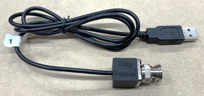
So, Figure 1 is the design I followed through on. The only thing to add to this is a BNC connector, an enclosure (with 4 screws), and a USB cable to power the unit. This simple design, and the fact that the IC is a tiny SOT-23 package, allows for a very small design as seen in Figure 2.
 |
|
| Figure 2. | The Tiny Pulser prototype with a 3D printable enclosure based on the schematic in Figure 1 that is roughly the size of a sugar cube. |
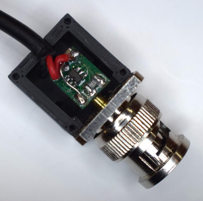
The 3D printable enclosure is roughly the size of a sugar cube, so I named the device the “Tiny Pulser”. Figure 3 shows the PCB in the enclosure while Figure 4 displays the PCB assembly.
 |
|
| Figure 3. | The PCB enclosure of the Tiny Pulser showing the BNC, IC, and passives used in Figure 1. |
The PCB is a 6 pin SOT-23 adapter available from various sources. As you can see in Figure 4, there are only a few things to solder to the PCB including a jumper. Three wires are attached including the +5 V and ground from the USB cable. The other ground wire needs to be soldered to the BNC body. To do this, I had to break out the old Radio Shack 100 W soldering gun to get enough heat on the BNC base by the solder cup. Scratching up the surface also helped. The PCB is then attached to the BNC by soldering the output pad of the PCB (backside) to the BNC solder cup.
 |
|
| Figure 4. | Tiny Pulser 6-pin SOT-23 PCB assembly with only a few components and jumper wires to solder to the PCB itself. |
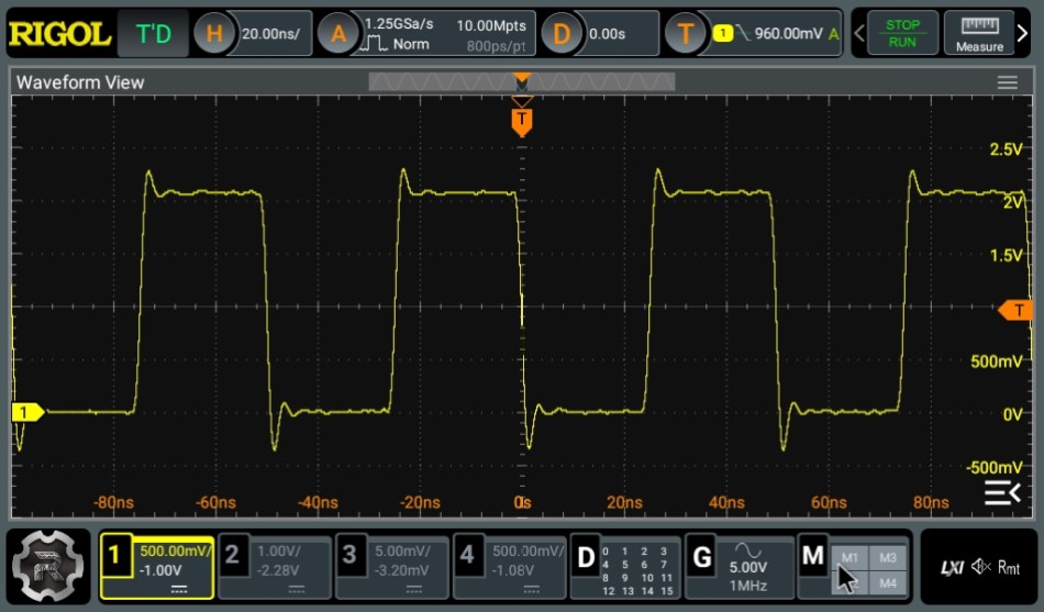
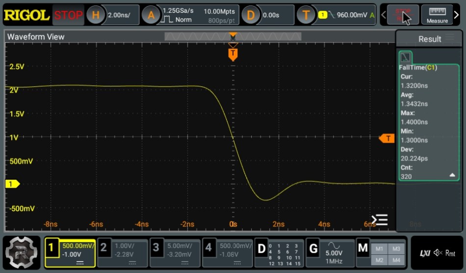
So how does it perform? The best performance is obtained when using a 50 Ω scope input and measuring the fall time which was a bit faster than the rise time. In Figure 5 we see the generated pulse train of 20 MHz while Figure 6 is a screenshot showing a fall time of 1.34 ns.
 |
|
| Figure 5. | The generated pulse train of 20 MHz of the Tiny Pulser using a 50 Ω scope input. |
 |
|
| Figure 6. | Fall time measurement (1.34 ns) of the Tiny Pulser circuit made on a 50 Ω scope input. |
You can see the pulse train is pretty clean with a bit of overshoot. Note that the 1.34 ns fall time is a combination of the scopes fall time and the Tiny Pulsers fall time. Now we need to figure out the actual fall time of the Tiny Pulser.
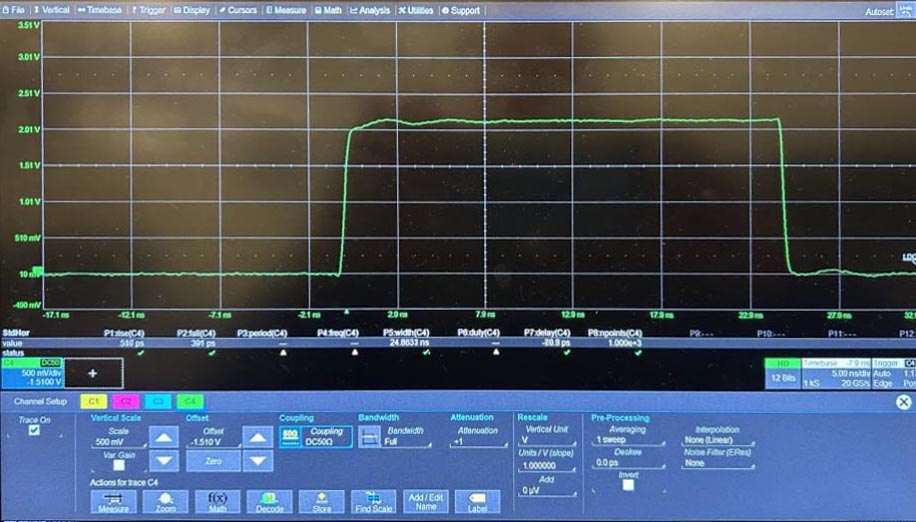
As I said I got a chance to use a high-powered scope (2.5 GHz, 20 GS/s) to measure the rise and fall times. Figure 7 shows the results (pardon the poor picture).
 |
|
| Figure 7. | Picture of the high-end oscilloscope (2.5 GHz, 20 GS/s) display measuring the rise and fall times of the Tiny Pulser. |
You can see that the Tiny Pulser delivers a very clean pulse with a rise time of 510 ps and a fall time of 395 ps. We now have all the information we need to make our bandwidth calculations. (The formulas we have developed are as applicable to fall time as they are to rise time, so we will not change the variable names.)
Using the scopes measured fall time and the 395 ps Tiny Pulser fall time, we calculate the bandwidth of the scope, first by calculating the scopes maximum fall time [Equation (6)]:
 |
(7) |
And now use this to calculate the bandwidth [Equation (1)]:
 |
(8) |
A gut check tells me this is a reasonable number for an oscilloscope sold as a 250 MHz model.
I tested another scope I have that is rated as 200 MHz. It displayed a fall time of 1.51 ns which works out to be 240 MHz. This number agrees to within a few percent of other numbers I have found on the internet. It seems like the Tiny Pulser works well for measuring scope bandwidth!
Another use for a fast pulse
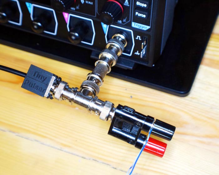
A better-known use for a fast rise time is probably in a time-domain reflectometer (TDR). A TDR is used to measure the length, distance to faults, or distance to an impedance change in a cable. To do this with the Tiny Pulser, add a BNC tee adapter to your scope and connect the cable (coax, twisted pair, zip cord, etc.), to be tested, to one side of the tee adapter (use a BNC to banana jack adapter if needed). Do not short the end of the wire. Next, connect the Tiny Pulser to the other side of the tee adapter as seen in the setup in Figure 8.
 |
|
| Figure 8. | A TDR set up using the Tiny Pulser with a BNC tee adapter to connect the circuit as required (e.g., via coax, twisted pair, etc.). |
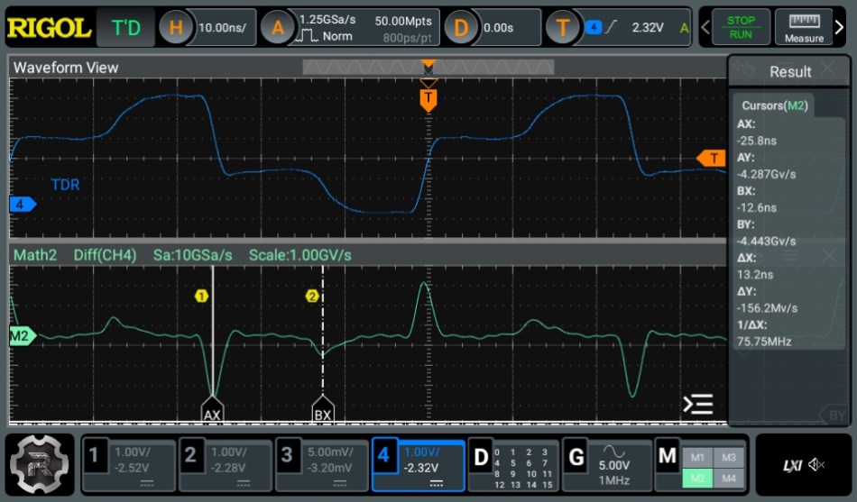
Now power up the Tiny Pulser and adjust the sweep rate to around 10 ns/div so you see something like the upper part of the screen in Figure 9. I find that the high impedance setting on the scope works better than the 50 Ω setting for the wire I was testing. This may vary with the wire you are testing. You can see that the square wave is distorted which is due to the signal reflecting from the end of the wire. If your scope has a math function to display the derivative (or differential) of the trace you will be able to see what’s happening clearer. This can be seen in the lower trace in Figure 9 when I connected a 53 inch piece of 24 AWG solid twisted pair.
To find the timing of the reflection, measure from the start of the pulse rising (or falling) to the distorted part of the pulse where it is rising (or falling) again. Or, if using the math differential function, measure the time from the tall bump to the smaller bump – I find this much easier to see.
In Figure 9 the falling edge of the pulse is marked by cursor AX and the reflected pulse is marked with the cursor BX. On the right side we can see the time between these pulses is 13.2 ns.
The length of the cable or distance to an impedance change can now be calculated but we first need the speed of the wavefront in the wire. For that we need the velocity factor (VF) for the cable that is being tested. This is multiplied by the speed of light to obtain the speed of the wavefront. The velocity factor for some cables may be found at Ref. 2.
In the case of Figure 9, the velocity factor is 0.707. Multiplying this with the speed of light in inches gives us 8.34 inches/ns. So, multiplying 13.2 ns by 8.34 inches/ns yields 110 inches. But this is the time up and down the wire, so we divide this by 2 giving us 55 inches. There are a few inches of connector also, so the answer is very close to the 53 inches of wire.
 |
|
| Figure 9. | Using the high impedance setting on the scope to perform a TDR test on a 53” piece of 24 AWG wire. The math function displays the derivative of the trace to view results more clearly. |
Note that, because we have a pulse rate of 20 MHz, we are limited to identifying the reflections up to about 22 ns, after which reflection pulses will blend with the next edge generated pulse. This is about 90 inches of cable.
One last trick
An interesting use of the TDR setup is to discover a cable’s impedance. Do this by adding a potentiometer across the end of the cable and adjust the pot until the TDR reflections disappear and the square wave looks relatively restored. Then measure the pot’s resistance and this is the impedance of your cable.
