At the end of the DI for a Simple log-scale audio meter (Ref. 1), I promised to show how to upgrade it to work better. With these fixes, it now has near-digital performance, with faster response and smoother operation. Even this supersized version comes in two flavours, one comparatively simple, the other, maxed out. It can now out-perform the standard peak program meter (PPM) specs (for which Ref. 2 a good reference), and has a span of over 60 dB with easy setting of the desired minimum and maximum levels.
While the goal for the original version was to produce something simple and functional, the aim of this DI is to see how closely we can match the performance of a few lines of DSP code, no matter how much hardware it may take. The original used just one dual op-amp; this approach inflates that to two quad packs. Over the top: of course. Instructive fun: definitely, at least for us analogeeks.
The underlying principle is the same as before – force current through a diode, measure the resulting voltage, which is proportional to the logarithm of the input, and capture the peak value – but the implementation is different. Figure 1 shows the basic circuit.
 |
|
| Figure 1. | We take the log of the input signal; its peak level is captured on C2, which is discharged slowly and linearly; and temperature- and level-corrections are applied in the current source which drives the meter. |
The audio input to be measured is now applied through R1, a 10k fixed resistor rather than a thermistor. The thermistor gave compensation for the diodes’ tempco by scaling the (linear) input; with the fixed resistor, we’ll apply an offset to the (logged) signal later in the circuit to achieve the same result. A1’s output is a logarithmically-squashed version of the input. For now, we only need its positive peaks.
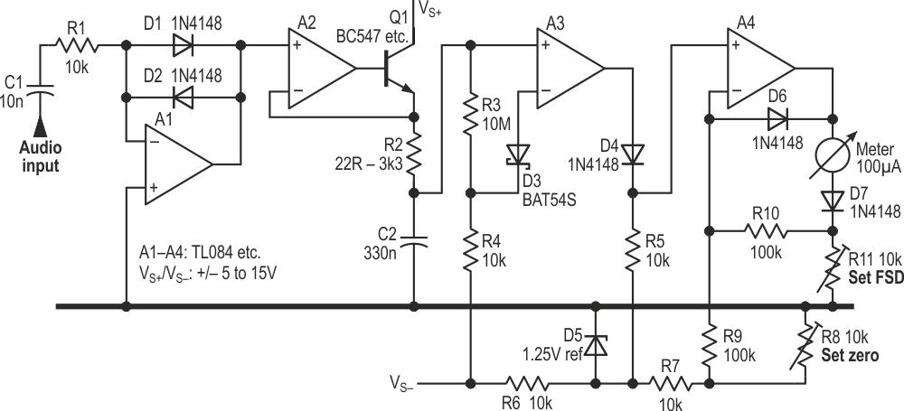
A2 and Q1 form a simple peak detector. Whenever A1.OUT is greater than the voltage on C2, A2/Q1 dumps current into C2 until the voltages match. Using a transistor rather than a diode greatly improves the speed; as drawn, with R2 = 22R, it will capture a single half-cycle at 20 kHz, as shown in Figure 2 which is way faster than the PPM spec calls for. (For a slower, more realistic response, increase R2. 1k5 gives a ~5 ms response time to within 1 dB of the final reading.) This may seem to be several op-amps short of a “proper” peak detector, but it does the job in hand: it’s been Muntzed. (Muntz? Who he? This (Ref. 3) will explain.) Taking A2.IN- directly from C2, which might seem more usual, leads to overshoot or slows the response, depending on the value of the series resistor.
 |
|
| Figure 2. | The attack or integration time is very fast; the decay or return time, much slower, and linear. |
Now that we have charged C2 fast, we need to discharge it slowly. A3 buffers its voltage, with D3/R4 bootstrapping R3 to give a linear fall in voltage equivalent to 20 dB in 1.7 s, which, more by happy accident than by design, is exactly what we want.
Now we pass the signal through D4, whose tempco of about –2 mV/°C compensates for that of D1/2. It also drops the level by its VF of about 600 mV, which needs restoring. D5 is shown as a generic 1.25 V shunt stabiliser, and its exact type or value is not critical. (I used an LM385 which was to hand; with a clean, stable negative supply rail, it can be designed out.) It provides an accurate source for offsetting not only D4’s VF, but also the signal as a whole, to set the meter needle’s zero point. R8 allows adjustment of this from about –62 dBu (R8 = 10k) to +1 dBu (R8 = zero).
A4 drives the meter movement, buffering the voltage from D4, the offset-voltage compensation being applied through R9. A4 drives current through the meter into R11, the resulting voltage across that being fed back through R10 to close the feedback loop. The meter has D7 in series with it to prevent underswings, and D6 catches negative swings on A4. (Shame we can’t do the same for A2.)
Calibration is simple. Apply the minimum input level at the input, or apply a DC voltage corresponding to the minimum negative peak value to the signal end of R1, and adjust R8 for zero indication on the meter. Now apply the maximum level – I chose +10 dBu – and set R11 for full-scale deflection. R8 must be set first, then R11.
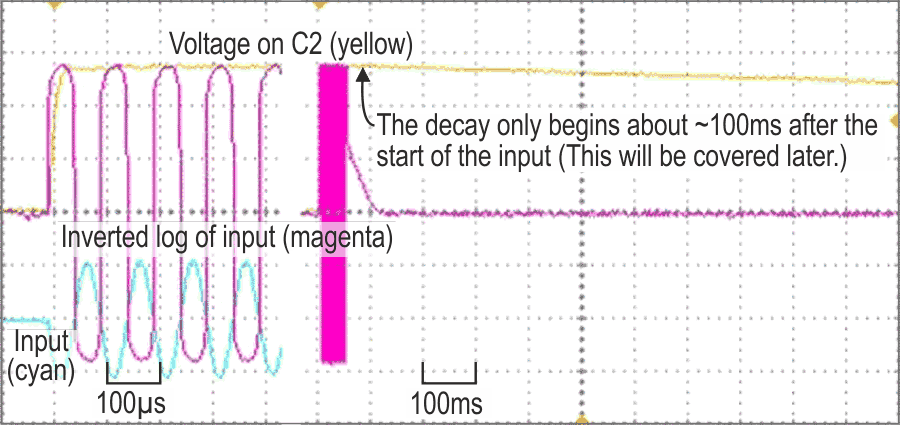
Temperature stability is good. According to LTspice, the tempco is zero at around +1 dBu input and reasonable at other levels, giving a reading correct within 1 dB down at –50 dB or so for 15 to 35 °C. Frustratingly, I could only get better compensation by adding extra resistors and a thermistor in a network around R10, the values differing according to the desired span: too many interactions. An extra stage could have fixed this, but… Figure 3 shows the response of the meter, both simulated and live.
 |
|
| Figure 3. | Simulated and measured responses when set up for a 50 dB span with a +10 dBu maximum reading, showing the effects of temperature and op-amp offset. |
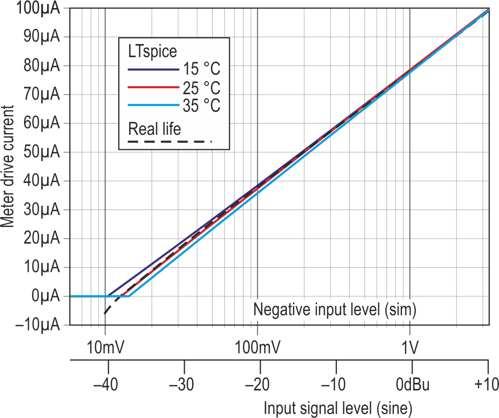
We now have a high-performance meter, with near-digital accuracy and even precision. But it’s still only half-wave sensing, and has a couple of residual bugs. For full-wave operation, we can add inverter A5, etc., to the output of A1, along with a second peak-detection stage, A6 and Q2, effectively paralleled with A2 and Q1, to add in the contribution from positive-going inputs: see Figure 4. If A1 and A5 have zero offset voltage or if a few trimmer-derived millivolts are applied to A2.IN+ and A5.IN+, C3 can be omitted. The input offsets inherent in real-world (and cheap) op-amps limit the span, as they lead to inaccuracies at low levels, where the signal to be measured is comparable with them.
 |
|
| Figure 4. | Extra components can be added for full-wave detection. |
Another way of adding bipolar detection would have been to use a full-wave rectifier at the input, but the extra op-amp offsets made this approach too inaccurate without messy trimming.
This circuit responds faster than a meter movement can follow. C2 may be charged almost instantaneously by a transient, but its voltage will decay by an indicated 11.8 dB/second (or 20 dB in 1.7 s). Thus, if the meter takes 85 ms to respond, it will under-read that transient by 1 dB. Figure 5 shows how to cure this.
A7 and A8 form a monostable, which is triggered by a sharp increase in C2’s voltage and generates a positive pulse at A7.OUT. Connecting this to R4, which no longer goes to VS–, via a diode cures the problem: while A7.OUT is low, C2 will discharge in the normal way, but while it is high, C2’s discharge path is effectively open-circuited. As shown, and with ±6 V rails, this hold time is ~100 ms. Adjust C5 or R16 to vary this. The result can be seen in Figure 2.
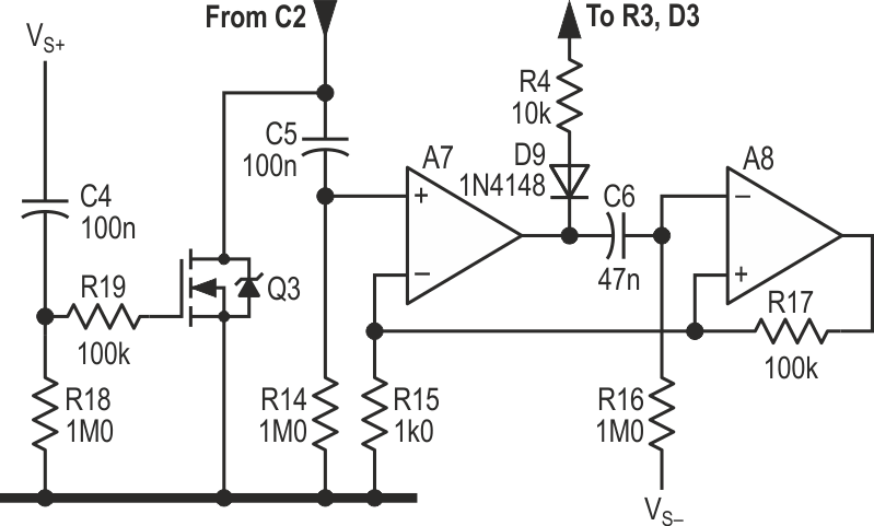 |
|
| Figure 5. | Final additions: a “power-on reset”, and a monostable to give ~100 ms hold time after a peak to allow the meter movement to catch up. |
A final touch is a power-on reset, also shown in Figure 5. (Digital circuits usually have them, so why should we be left out?) A sharp rise of the positive rail turns on Q3 – which may be almost any n-MOSFET – for a few hundred milliseconds, clamping C2 to ground while the circuitry stabilises. Without this, C2 may charge to a high level at power-on, taking many seconds to recover.
Although a 100 µA meter movement is shown, A4 will comfortably drive several milliamps. Select or adjust R11 to suit.
While you may not want to build a complete meter like this, the techniques and ideas used here may well come in handy for other projects. But if you do, be sure to use an ebonite-cased movement, complete with polished brass inlays, and with a pointer based on a Victorian town-hall clock’s minute hand. Electro-punk lives!
