This Design Idea has proved as useful as it is simple. With just three or four components, it allows the monitoring of current from microamps to well over 100 mA in a single range.
I was developing a PIC-based board and needed to monitor the current it drew from a pair of AA cells. Although spending most of its time asleep, with the boost converter’s 30 µA quiescent current dominating consumption, the board could cycle rapidly through bursts of sensing, displaying, and transmitting, drawing from 8 mA to 100 mA. Trying to use a DMM on fixed ranges was frustrating, while auto-ranging just gave me a headache owing to the fast cycling times and short on-periods. Thus, the following approach suggested itself.
The voltage across a diode increases as the logarithm of the current flowing through it, as defined by the diode equation:
where
IF is the forward current
I0 is the reverse saturation current
e is the electron charge (1.602 × 10⁻¹⁹ C)
VF is the forward voltage
T is the temperature (K)
k is Boltzmann’s constant (1.380 × 10⁻²³ J/K).
(This is a slightly stripped-down engineer’s version; for the full works and useful links, see reference 1.) For our purposes, we can extract from it:
VF ∝ logIF
at a given temperature.
Now, shunt a diode with a meter movement. At very low currents, it will indicate microamps as the current flows through it rather than the diode, while at high currents it will show the voltage across the diode and thus the log of the current (think of the diode as an adaptive shunt). Thus, the bottom of the meter scale is reasonably linear, the top is adequately logarithmic, the middle is transitional, while the whole is very useful.
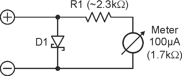
Using a Schottky rectifier, a 100 µA/1.7 kΩ meter, and a suitable series resistor as shown in Figure 1 allows the monitoring of currents from 10 µA to over 100 mA in a single range, with the speed of indication being limited only by the meter’s ballistics.
 |
||
| Figure 1. | ||
Anything this simple usually has more problems than components! Apart from a fiddly calibration procedure (more below), this circuit has two main flaws: its series voltage drop, and its temperature stability. The diode will drop up to 400 mV, so use new or fully-charged cells when monitoring, or your UUT may see the battery as low. Alternatively, think of this as a handy low-battery-sense-testing feature, perhaps adding a shorting switch.
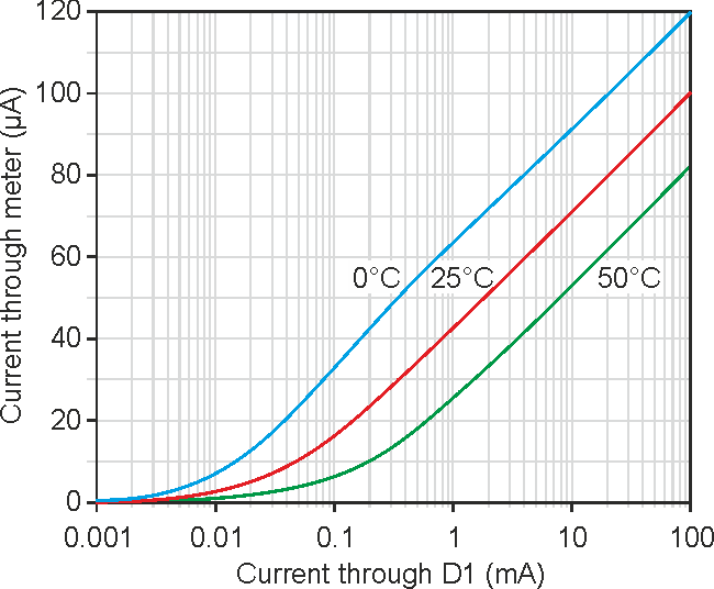
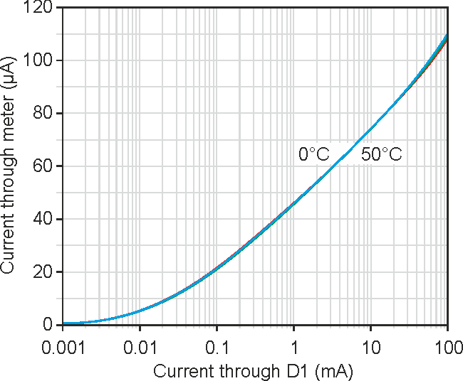
At the bottom of the scale, with almost all current flowing through the meter, the measurement tempco is low, being limited to the mechanical and magnetic temperature coefficients of the meter movement. At higher currents though, we are seeing the voltage across the diode, which of course decreases by about 2 mV/K as predicted by the diode equation. This not only affects the slope of the log law, but also our linear-to-log transition point. In addition, the meter winding forms a significant part of the total series resistance, copper having a TCR of +3930 ppm/K at room temperature. The resulting deflection vs. current curves shown in Figure 2 are for a 1N5817 at temperatures of 0°, 25°, and 50 °C. These account for the movement’s TCR as well as the tempco of the diode, but ignore any self-heating effects in the latter. At a fairly constant temperature there is no practical problem.
 |
||
| Figure 2. | ||
Self-heating, mainly in D1, is no real problem either. Let’s assume that 100 mA is flowing and that D1 is dropping 400 mV: that’s 40 mW. The DO-41 1N5815 has a basic thermal resistance of 50 K/W according to its data sheet – with longish leads and lots of heat-sinking copper. Putting these figures together shows that at 100 mA, the junction will rise by just 2°, equivalent to a decrease in VF of about 4 mV, or about 1% error at full scale. Try to keep your diode’s leads short and your thermal masses high. Beware of high transient currents, perhaps at switch-on, as these will cause errors until the junction cools down again.
 |
||
| Figure 3. | ||
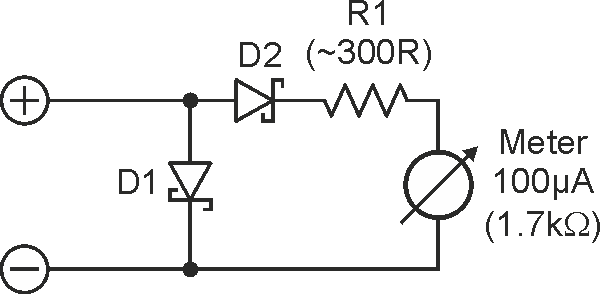
The improved version in Figure 3 nulls the tempco by adding an extra diode in series with the meter movement; its curves shown in Figure 4. Note that the bulk of the scale is now log-ish, the extra diode effectively suppressing the initial, linear region. However, the choice of diodes is now critical, as D2 should have a slightly lower forward voltage than D1 but matching characteristics otherwise. Confusing.
 |
||
| Figure 4. | ||
LTspice to the rescue! I hit on the combination of a 10MQ060N for D1 and a BAT54 for D2 by happy accident – it was the first pair I simulated. Both are cheap, available, and modelled natively by LTspice, so they are therefore recommended. A pair of 10MQ060Ns works almost identically (but a pair of BAT54s doesn’t). Combinations of other devices mostly show worse temperature variations with kinkier indications, so model before you build. R1 could be omitted if the meter’s sensitivity and resistance are suitable. Couple D1 and D2 together thermally so they will track one another with temperature.
Silicon P-N junction diodes generally have very straight (log IF)/VF relationships; Schottkys don’t. This is due to their construction, which has an inherently higher series resistance, causing the law to become more linear than log at very low currents, and often also has guard rings to control potential gradients, which can form P-N diodes paralleled with the Schottky junction itself, thus softening the curve at high currents. So in practice, the precise log law varies with current as well as device type. So while a junk-box diode may be fine for the first version – given that circuit’s unavoidable inaccuracies – careful selection is needed for the two-diode design. Reference 2 gives more background.
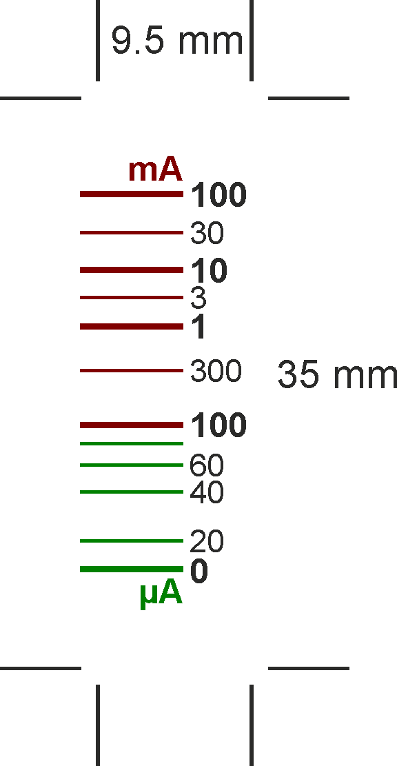
Because I have a box of cheap leftover edgewise 100 µA/1700 Ω indicators that fit 35×14 mm apertures, I use those. This type is very common and gives a compact, practical result, but their construction, linearity, and consistency between units would make the ghost of Monsieur d’Arsonval weep.
 |
||
| Figure 5. | ||
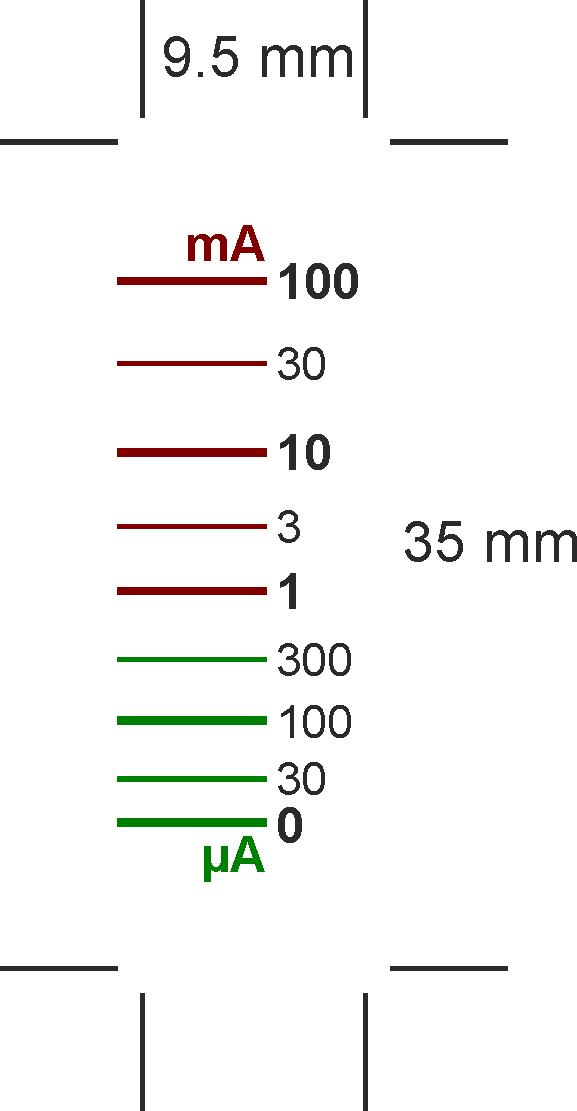
The calibration points used in Figure 5 were generated by arranging series combinations of the monitor, a battery, fixed and variable resistors, and a DMM. The existing meter scale was marked at suitable points, then removed and scanned, the scan being used as a template for the final layout. The simulation results were used to generate the datum points for Figure 6, but the results reflect reality well, despite the horrible meter. These scales will save you time but won’t be quite as accurate as making your own from scratch (obviously, other movements will need different scales). Adjust R1 to trim the calibration (the meter is specified as ±20%). Both scales take the movement’s nonlinearity into account.
 |
||
| Figure 6. | ||
Note that I call this a “monitor” rather than a “meter”; the latter term implies, to me, something with better accuracy. Nonetheless, I now build these into most of my development and even production test rigs, and very useful they are for spotting a variety of faults and problems, from shorted power traces to wrongly-coded pullup pins.