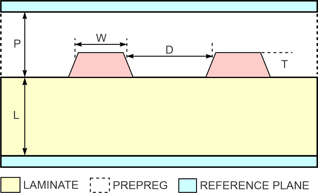
Differential signaling is a common technique for obtaining high noise immunity for critical signals in high-speed digital pc-board systems. The pc board's traces, carrying differential signals, are often edge-coupled offset striplines, with the traces sandwiched between two reference planes (Figure 1). Striplines are desirable because they offer good protection against EMI and ESD and because they allow you to tightly control tolerances in fabrication.
 |
|
| Figure 1. | PSpice can model edge-coupled offset striplines for impedance and propagation delay. |
Unfortunately, PSpice does not provide a geometry-characterized model of two edge-coupled striplines that carry differential signals. As a result, when it is necessary to simulate a differential stripline, you must use the PSpice Tline-coupled model with the line parameters (L, C, Lm, Cm) obtained by means of a 2-D field solver. Listing 1 shows the PSpice subcircuit that represents the model of two lossless, differentially routed striplines, as in Figure 1.
Listing 1. PSpice model for differential stripline
SUBCKT diff_stripline al a2 bl b2 params: W=lu D=lu T=lu L=lu P=1 kc=l
+ er=4.6LEN=l
.func Pi() (4*atan(l)}
.func A(x) {1+log(1+1/tanh(Pi()*D/(4*x+2*T)))/log(2)}
.func C(x) {2*log(2+T/(2*x))-(T/(2*x+T))*log(T*(4*x+T)/(4*x**2))}
.func Zl(x) {60*Pi()*x/((sqrt(kc*er))*(W+(2*x+T)*C(x)*A(x)/(2*Pi())))}
T_T1 al 0 bl 0
+Z0={2*Z1(L)*Z1(P-T)/(Z1(L)+Z1(P-T))}
+TD={(sqrt(er)/3.0e8)*LEN}
T_T2 a2 0 b2 0
+Z0={2*Z1I(L)*Z1(P-T)/(Z1(L)+Z1(P-T))}
+TD={(sqrt(er)/3.0e8)*LEN}
.ENDS diff_stripline
You can use the subcircuit for both transient and ac analysis. The model's input parameters are the geometrical dimension of the striplines in meters; the relative permittivity, εr, of the surrounding medium; the trace length in meters; and the correction factor, kc (Reference 1). The model calculates the odd-mode impedance of each stripline (in other words, the impedance of a single stripline when the two striplines carry differential signals) with a maximum error of 5 to 6%. The model also calculates the propagation delay. The odd-mode impedance of each line is the parallel combination of two odd-mode impedances, each one calculated with respect to each reference plane. The empirically determined correction factor, kc, takes into account the imperfection of the formulas in the model in determining the odd-mode impedance of each line. The correction factor is a function of the pc-board material and its supplier.