In this Design Idea (DI), the classic Schmitt-trigger-based RC oscillator is “hacked” and analyzed using the simulation software QSPICE (Ref. 1). You might reasonably ask why one would do this, given that countless such circuits reliably and unobtrusively clock away all over the world, even in space.
Well, problems arise when you want the RC oscillator to be tunable, i.e., replacing the resistor with a potentiometer. Unfortunately, the frequency is inversely proportional to the RC time constant, resulting in a hyperbolic response curve.
Another drawback is the limited tuning range. For high frequencies, R can become so small that the Schmitt trigger’s output voltage sags unacceptably.
The oscillator’s current consumption also increases as the potentiometer resistance decreases. In practice, an additional resistor ≥1 kΩ must always be placed in series with the potentiometer.
The potentiometer’s maximum value determines the minimum frequency. For values >100 kΩ, jitter problems can occur due to hum interference when operating the potentiometer, unless a shielded enclosure is used.
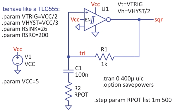
RC oscillator
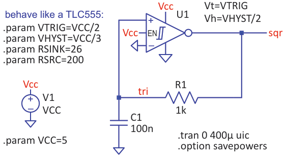
Figure 1 shows an RC oscillator modeled with QSPICE’s built-in behavioral Schmitt trigger. It is parameterized as a TLC555 (CMOS 555) regarding switching thresholds and load behavior.
 |
|
| Figure 1. | An RC oscillator modeled with QSPICE’s built-in behavioral Schmitt trigger, it is a TLC555 (CMOS 555). |
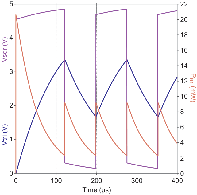
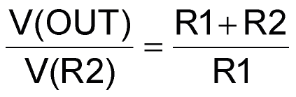
Figure 2 displays the typical triangle wave input and the square wave output. At R1 = 1 kΩ, the output voltage sag is already noticeable, and the average power dissipation of R1 is around 6 mW, roughly an order of magnitude higher than the dissipation of a low-power CMOS 555.
 |
|
| Figure 2. | The typical triangle wave input and the square wave output, where the average power dissipation of R1 is around 6 mW. |
Frequency response wrt potentiometer resistance
Next, we examine the oscillator’s frequency response as a function of the potentiometer resistance. R1 is simulated in 100 steps from 1 kΩ to 100 kΩ using the .step param command.
The simulation time must be long enough to capture at least one full period even at the lowest frequency; otherwise, the period duration cannot be measured with the .meas command.
However, with a 3-decade tuning range, far too many periods would be simulated at high frequencies, making the simulation run for a very long time.
Fortunately, QSPICE has a new feature that allows a running simulation to be aborted, after which the new simulation for the next parameter step is executed. The abort criterion is a behavioral voltage source called AbortSim(). It’s not the most elegant or intuitive feature, but it works.
Schmitt trigger oscillator
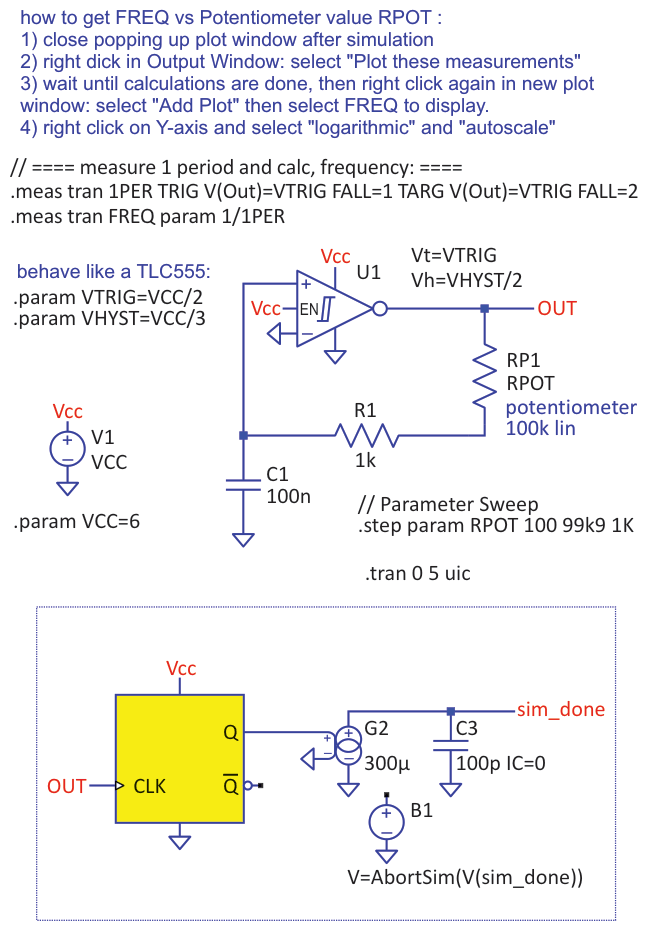
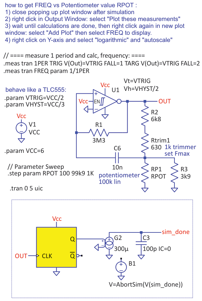
Figure 3 shows our Schmitt trigger oscillator, but this time with the parameter stepping of R1, the .meas commands for period and frequency measurement, and an auxiliary circuit that triggers AbortSim(). My idea was to build a counter clocked by the oscillator. After a small number of clock pulses – enough for one period measurement – the simulation is aborted.
 |
|
| Figure 3. | Schmitt trigger oscillator, this time, with the parameter stepping of R1, the .meas commands for period and frequency measurement, and an auxiliary circuit that triggers AbortSim(). |
I first tried a 3-stage ripple counter with behavioral D-flops. This worked but wasn’t optimal in terms of computation time.
The step voltage generator in the box in Figure 3 is faster and easier to adjust. A 10-ns monostable is triggered by V(OUT) of the oscillator and sends short current pulses via the voltage-controlled current source to capacitor C3. The voltage across C3 triggers AbortSim() at >= 0.5 V.
The constant current and C3 are selected so that the 0.5 V threshold is reached after 3 clock cycles of the oscillator, thus starting the next measurement.
Note that the simulation time in the .tran command is set to 5 s, which is never reached due to AbortSim().
The entire QSPICE simulation of the frequency response takes the author’s PC a spectacular 1.5 s, whereas previously with LTspice (without the abort criterion) it took many minutes.
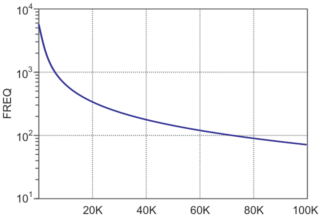
Figure 4 shows the frequency (FREQ) versus potentiometer resistance (RPOT) curve in a log plot, interpolated over 100 measurement points.
 |
|
| Figure 4. | Frequency versus potentiometer resistance curve in a log plot, interpolated over 100 measurement points. |
Final circuit hack
Now that we have the simulation tools for fast frequency measurement, we finally get to the circuit hack in Figure 5. We expand the circuit in Figure 1 with a resistor R2 = RPOT in series with C1.
 |
|
| Figure 5. | Hacked Schmitt trigger oscillator with an expanded Figure 1 circuit that includes R2=RPOT in series with C1. |
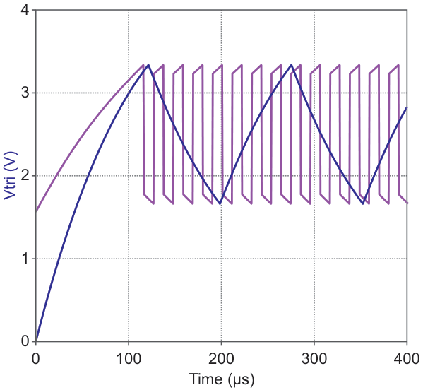
Figure 6 illustrates what happens: for R2 = 0 (blue trace), we see the familiar triangle wave. When R2 is increased (magenta trace), a voltage divider:
is created if we momentarily ignore V(C1). V(R2) is thus a scaled-down V(OUT) square wave signal, to which the V(C1) triangle wave voltage is now added.
 |
|
| Figure 6. | The typical triangle wave input with the output now reaching very high frequencies without excessively loading V(OUT). |
Because the upper and lower switching thresholds of the Schmitt trigger are constant, V(C1) reaches these thresholds faster as V(R2) increases. The more V(R2) approaches the Schmitt trigger hysteresis VHYST, the smaller the V(C1) triangle wave becomes, and the frequency increases.
At V(R2) = VHYST, the frequency would theoretically become infinite. This condition in the original circuit in Figure 1 would mean R1 = 0, leading to infinitely high I(OUT). The circuit hack thus allows very high frequencies without excessively loading V(OUT)!
The problem of the steep frequency rise towards infinity at the “end” of the potentiometer still remains. To fix this, we would need a potentiometer that changes its value significantly at the beginning of its range and only slightly at the end. This is easily achieved by wiring a much smaller resistor in parallel with the potentiometer.
Fixing steep frequency rise
In Figure 7, we see a second hack: R1 has been given a very large value.
 |
|
| Figure 7. | Frequency versus potentiometer resistance curve in a log plot, interpolated over 100 measurement points, showing a flatter curve profile and larger tuning range. |
This keeps the circuit’s current consumption low, especially at high frequencies. The square wave voltage at RPOT is now taken directly from V(OUT) via a separate voltage divider. This allows RPOT to be dimensioned independently of R1.
In the example, I used a common 100 kΩ potentiometer. The remaining resistors are effectively in parallel with the potentiometer regarding AC signals and set the desired characteristic curve.
Despite all measures, the frequency increase is still quite steep at the end of the range, so a 1 kΩ trimmer Rtrim1 is recommended for practical application to conveniently set the maximum frequency.
Figure 8 shows the frequency curve of the final circuit. Compared to the curve of the original circuit in Figure 4, a significantly flatter curve profile is evident, along with a larger tuning range.
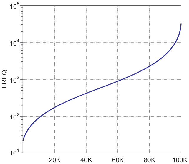 |
|
| Figure 8. | Frequency versus potentiometer resistance curve in a log plot, interpolated over 100 measurement points, showing a flatter curve profile and larger tuning range. |