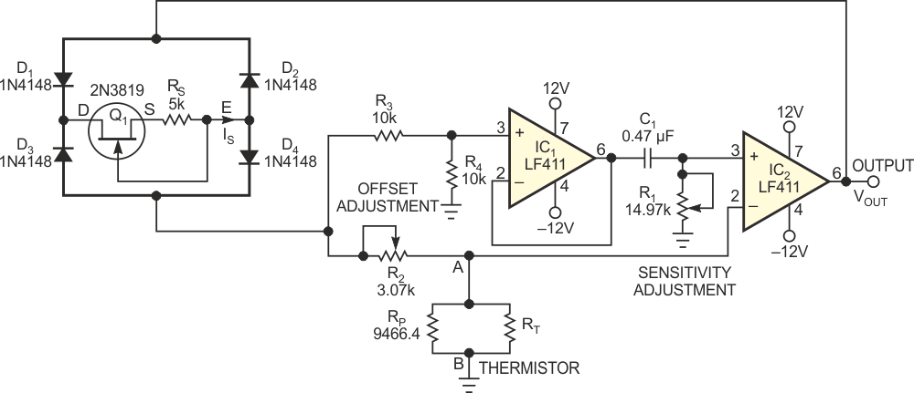
Designers often use thermistors rather than other temperature sensors because thermistors offer high sensitivity, compactness, low cost, and small time constants. But most thermistors' resistance-versus-temperature characteristics are highly nonlinear and need correction for applications that require a linear response. Using a thermistor as a sensor, the simple circuit in Figure 1 provides a time period varying linearly with temperature with a nonlinearity error of less than 0.1 K over a range as high as 30 K. You can use a frequency counter to convert the period into a digital output. An approximation derived from Bosson's Law for thermistor resistance, RT, as a function of temperature, θ, comprises RT = AB–θ (Ref. 1). This relationship closely represents an actual thermistor's behavior over a narrow temperature range.
 |
||
| Figure 1. | This simple circuit linearizes a thermistor’s response and produces an output period that’s proportional to temperature |
|
You can connect a parallel resistance, RP, of appropriate value across the thermistor and obtain an effective resistance that tracks fairly close to AB–θ ≈ 30 K. In Figure 1, the network connected between terminals A and B provides an effective resistance of RAB ≈ AB–θ. JFET Q1 and resistance RS form a current regulator that supplies a constant current sink, IS, between terminals D and E.
 |
||
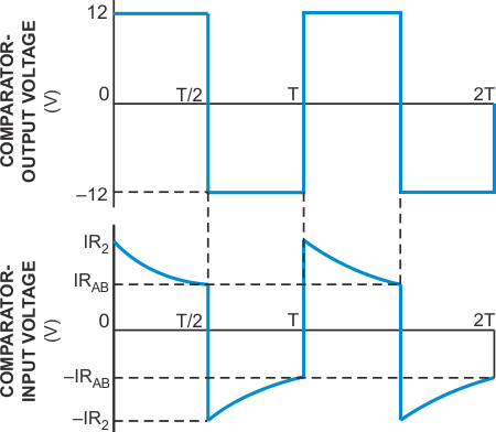
| Figure 2. | Waveforms show input to comparator IC2 (lower trace) and its output (upper trace). In the lower trace, IR2 represents the voltage across R2. |
|
Through buffer-amplifier IC1, the voltage across R4 excites the RC circuit comprising R1 and C1 in series, producing an exponentially decaying voltage across R1 when R2 is greater than RAB. At the instant when the decaying voltage across R1 falls below the voltage across thermistor RT, the output of comparator IC2 changes its state. The circuit oscillates, producing the voltage waveforms in Figure 2 at IC2's output. The period of oscillation, T, is

This equation indicates that T varies linearly with thermistor temperature θ.
You can easily vary the conversion sensitivity, ΔT/Δθ, by varying resistor R1's value. The current source comprising Q1 and RS renders the output period, T, largely insensitive to variations in supply voltage and output load. You can vary the period, T, without affecting conversion sensitivity by varying R2. For a given temperature range, θL to θH, and conversion sensitivity, SC, you can design the circuit as follows: Let θC represent the center temperature of the range. Measure the thermistor's resistance at temperatures θL, θC, and θH. Using the three resistance values RL, RC, and RH, determine RP, for which RAB at θC represents the geometric mean of RAB at θL and θH. For this value of RP, you get RAB exactly equal to AB–θ at the three temperatures, θL, θC, and θH.
At other temperatures in the range, RAB deviates from AB–θ, causing a nonlinearity error that is appreciably less than 0.1 K for most thermistors when the temperature range is 30 K or less. You can easily compute RP using:

Because temperature-to-period-conversion sensitivity, SC, is

you can choose R1 and C1 such that
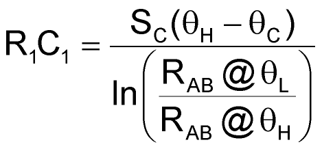
to obtain the required value of SC. To get a specific output period, TL, for the low temperature, θL, R2 should equal (RAB at θL)eY, in which
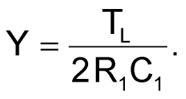
In practice, use a lower value for R2 because the nonzero response delay of IC2 causes an increase in the output period.
Next, set potentiometers R1 and R2 close to their calculated values. After you adjust R1 for the correct SC, adjust R2 until T equals TL for temperature θL. The two voltage-divider resistances, R3 and R4, should be equal in value and of close tolerances. As a practical example, use a standard thermistor, such as a Yellow Springs Instruments 46004, to convert a temperature span of 20 to 50 °C into periods of 5 to 20 msec. This thermistor exhibits resistances for RL, RC, and RH of 2814, 1471, and 811.3 Ω, respectively, at the low, midpoint, and high temperatures. Other parameters for the design include SC = 0.5 msec/K, θL = 20 °C, θH = 50 °C, θC = 35 °C, and TL = 5 msec.
Because only a fraction of current IS is through the thermistor, IS should be low to avoid self-heating effects. This design uses an IS of approximately 0.48 mA, which introduces a self-heating error of less than 0.03 K for a thermistor's dissipation constant of 10 mW/K. Figure 1 illustrates the values of the components in the example. All resistors are of 1% tolerance and 0.25 W rating; use a polycarbonate-dielectric capacitor for C1.
Simulating various temperatures from 20 to 50 °C by replacing the thermistor with standard, 2814 to 811.3 Ω, 0.01%-tolerance resistors produces T values of 5 to 20 msec with a maximum deviation from correct readings of less than 32 µsec, which corresponds to a maximum temperature error of less than 0.07 K. Using an actual thermistor produces a maximum error of less than 0.1 K for a thermistor dissipation constant of 10 mW/K or less.
Exploring Bosson's Law and its equation
One cause of confusion you may encounter when reading the papers in the references involves authors’ use of different symbols to represent a variable or a constant while referring to a commonly known equation. Readers unfamiliar with Bosson’s Law and its accompanying equation can view the original paper (Reference 1), in which the authors state Bosson’s Law as:
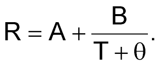
In the equation, quantities A, B, and θ represent certain thermistor constants, and temperature, T, is in kelvins.
By taking the exponent of both sides, you get
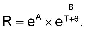
If you replace the constant eA with A, you can restate Bosson’s Equation as
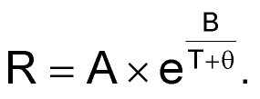
Most authors have used this form to represent Bosson’s Equation only in their published papers. Here, T is temperature, and θ is a constant.
Because T and θ come together in this equation as T+θ, you can alternatively use θ to represent temperature and T as a constant. The material in Reference 2 presents the equation as
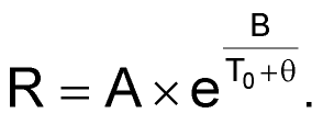
and denote it as Bosson’s Form. This equation uses T0 in place of T, and T0 is a constant. Reference B denotes the constant, T0, as initial temperature and θ as temperature.
With suitable assumptions, the literature derives the approximation R = AB–θ from the Bosson Form.
References
- Bosson, G, F Guttman, and LM Simmons, “A relationship between resistance and temperature of Thermistors,” Journal of Applied Physics , Volume 21, 1950, pg 1267.
- Yankov, IY, CI Gigov, and EA Yankov, “Linear temperature-to-time period converters using standard thermistors,” Measurement Science and Technology , Volume 1, No. 11, November 1990, pg 1168.