Frequent contributor Nick Cornford recently published a delightfully clever design idea (Reference 1) using a platinum RTD calibrated to output a 1 mV/°C signal that’s perfect for direct readout via a standard DMM…
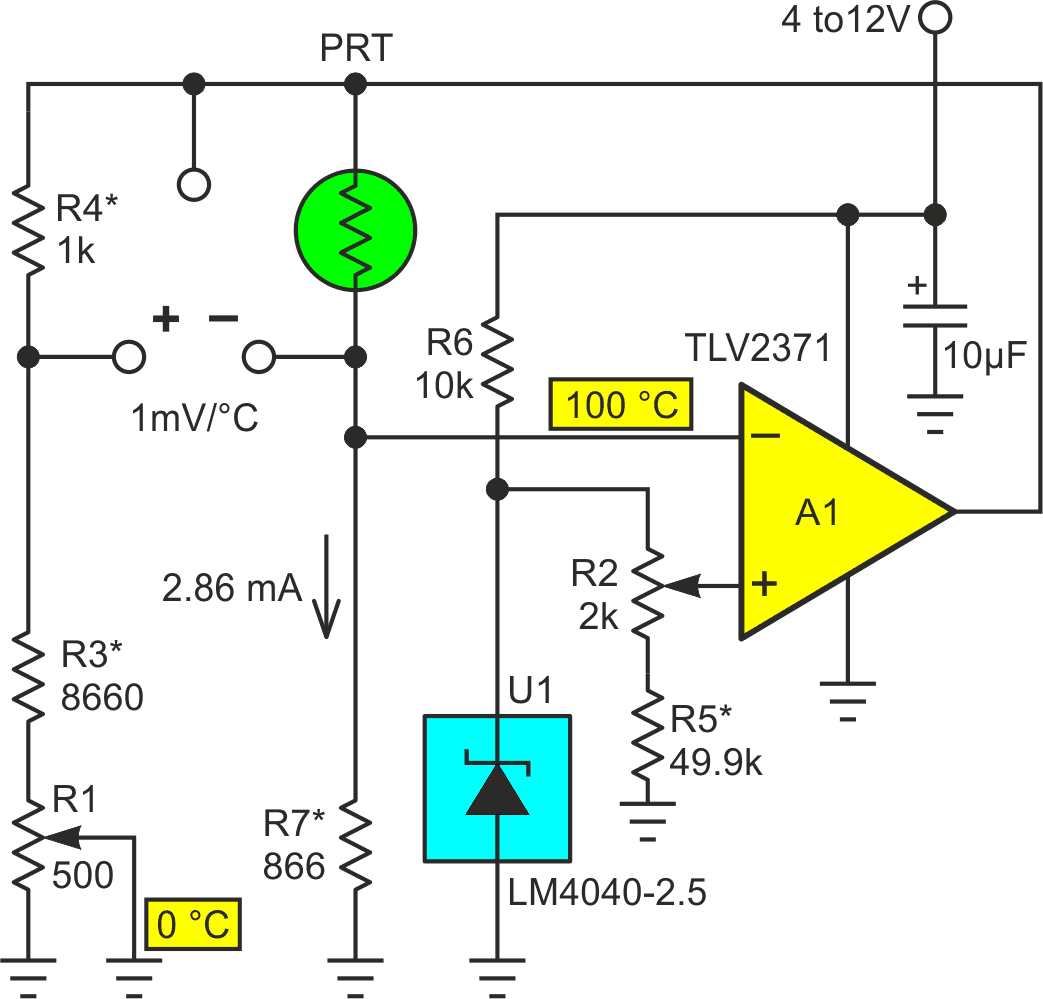
I thought Nick’s idea was so cool I just had to try and cobble up my own version of it. The initial effort is shown in Figure 1.
 |
|
| Figure 1. | PRTD circuit shamelessly copies Nick C’s idea for making an ordinary DMM into a precision digital thermometer. |
Figure 1’s circuit is conceptually identical to Nicks’s in putting the PRT into a basic bridge topology with constant current excitation of the PRT. It differs, however in one detail. Only the PRT half of the bridge is actively regulated with constant current while the other (zero adjust) half is just a passive voltage divider. This ploy reduces the parts count somewhat (saving two transistors, an op-amp, and maybe a resistor or two). But it doesn’t make the circuit work significantly worse or better. The calibration process is the same very-well-explained procedure in Nick’s DI as is achievable accuracy. I certainly won’t try to compete with Nick’s well written writeup in that regard.
In fact, I suppose you might legitimately ask if such a similar circuit really merits separate publication in the first place. Fortunately, this is not quite the end of our story.
Because of the 10% attenuation of the PRT signal inflicted by the passive side of my bridge, in order to duplicate Nick’s terrific feature of a 1 mV/°C direct-readout, I had to boost the PRT excitation current IPRT by that same 10% to make the bigger signal. So, I made

instead of the 2.597 mA used by Nick in his double-constant-current-source circuit. So far, so good.
But then this got me musing about what effect further multiples of IPRT might have. This was very interesting, of course, because platinum’s tempco is not exactly constant with temperature, a fact described by the Callendar-Van Dusen polynomial. It predicts platinum’s tempco declines steadily from the 0 °C value as temperature T increases. Note the pesky quadratic ‘B’ term.
R(T) = R(0)[1 + (A×T) – (B×T2)],
A = 3.9083×10⁻³,
B = 5.775×10⁻⁷.
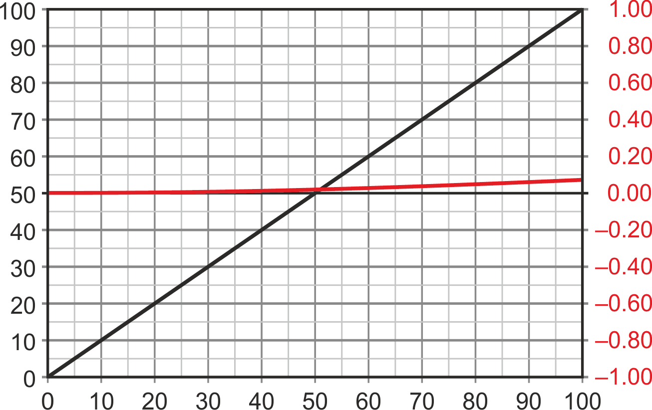
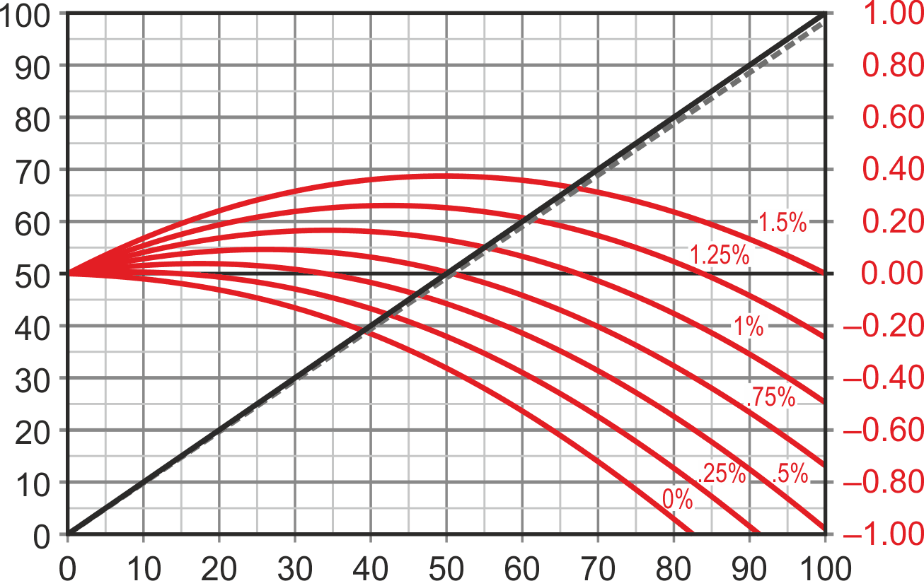
So, I calculated the circuit’s output over 0 °C to 100 °C while gradually bumping IPRT. The interesting results are plotted in Figure 2. X axis = actual temp, red = reading error in degrees.
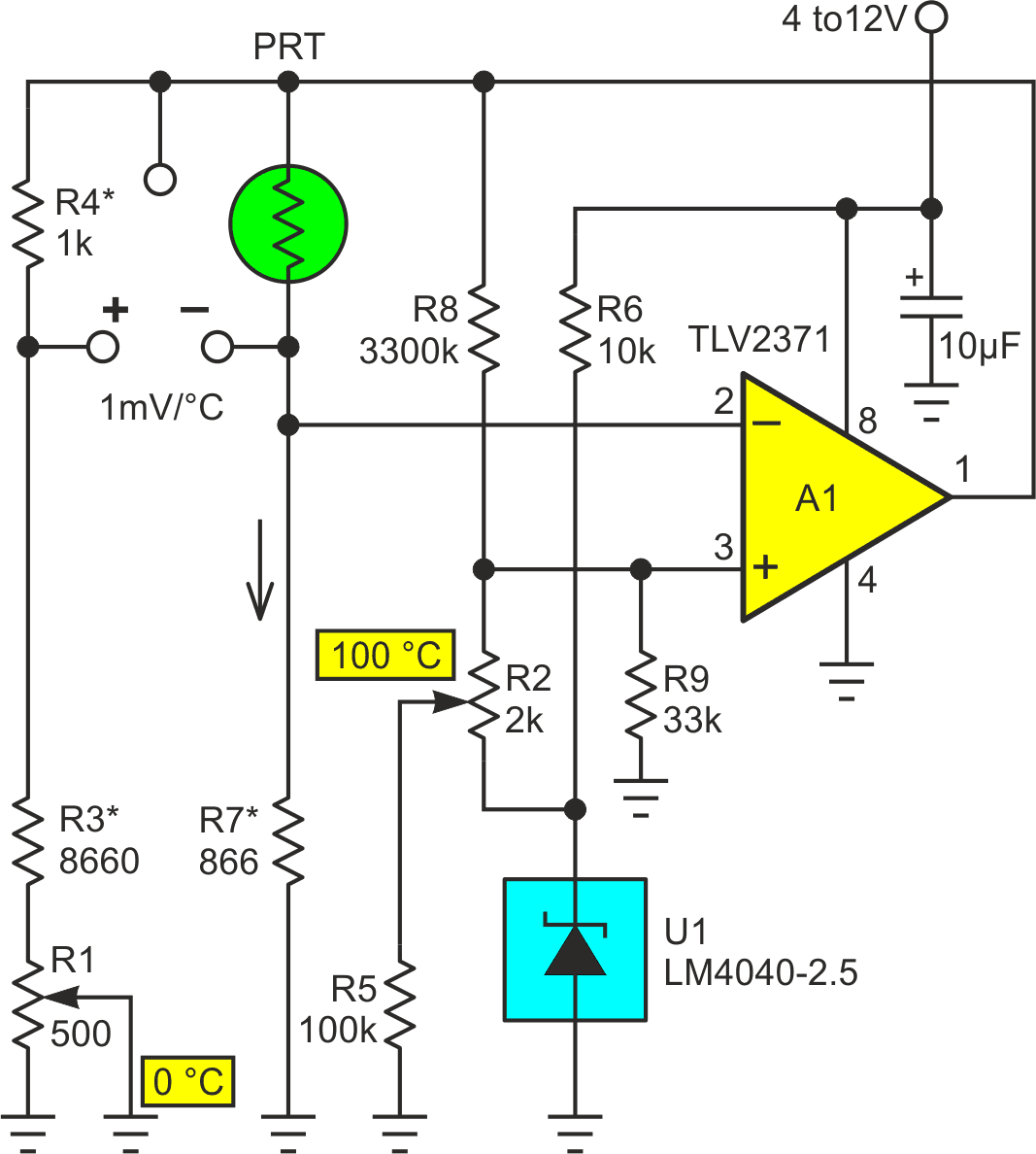
All that’s required to utilize this effect to continuously and automatically fix the reading is the addition of R8 and R9 to generate the positive feedback provided in Figure 3. Now:
IPRT(T) = IPRT(0)[1 + 0.15(VPRT(T) – VPRT(0)].
Thus, as the readout voltage goes from 0 to 100 mV, the IPRT excitation current increases by the 0 to +1.5% needed to accurately linearize the reading. The residual error with Figure 3’s positive feedback can be seen in Figure 4.
 |
|
| Figure 4. | Residual error with Figure 3’s positive feedback. |
And that, I thought, was worth its own write up. I hope Nick will agree.
Postscript
As per my usual habit, I did research on PRTD linearization with positive feedback only after I’d already blundered my way to this solution on my own. But having done it, I wanted to see if anybody else was using the method. Yes. They are.
Guess who (Ref. 2)? I’m actually now kind of glad I didn’t look before I leaped. If I’d already seen the complexity of Jim’s circuit, I might not have attempted it!
References
- Cornford, Nick. "DIY RTD for a DMM."
- Williams, Jim. "Signal Conditioning for Platinum Temperature Transducers."

