A self-heated Darlington transistor pair makes a simple, sensitive, and sturdy airflow sensor. But first an annoying non-linearity needs unbending.
If you take a self-heated transistor in a TO-92 package and force it to hold a constant temperature differential above ambient, the power input required to keep it stuck to setpoint will be determined by its thermal impedance ZT relative to the air, as given by:
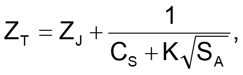
ZJ = junction-to-case thermal impedance = 44 °C/W;
CS = still-air case-to-ambient conductivity = 6.4 mW/°C;
K = “King’s Law” thermal diffusion constant = 0.75 mW/°C√fpm;
SA = air flow in ft/min.
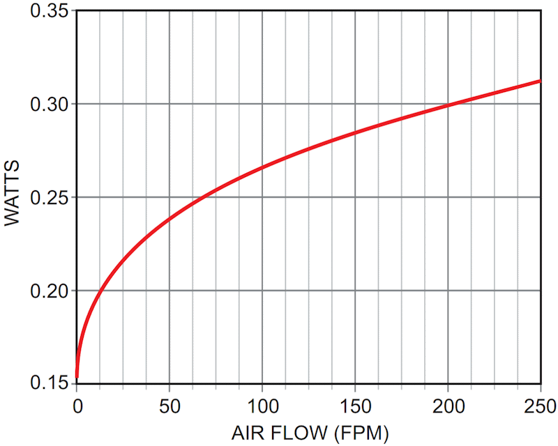
The SA term suggests the arrangement might be handy for air flow measurement, because of the way it makes ZT, and therefore power input for a given differential, a function of air speed. Figure 1 shows the resulting power vs SA relation a differential (Dt) = 31 °C. Do note, however, the annoying non-linearity.
 |
|
| Figure 1. | This graph shows the power dissipated vs air speed of a TO-92 held at a constant 31 °C above ambient PW = 31/ZT. |
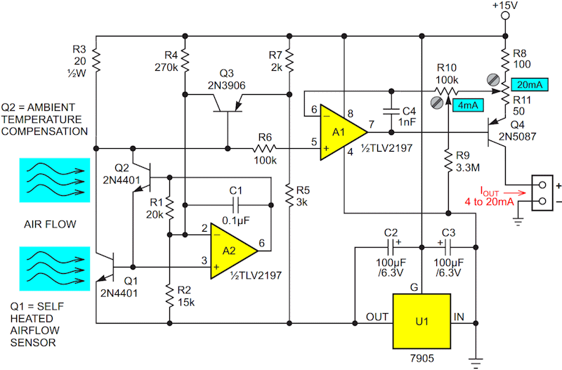
Figure 2 shows a practical thermostat circuit to achieve and maintain this delta-T while outputting a signal predictably related to PW. It utilizes a Darlington sensor transistor pair (Q1 and Q2) to compensate for ambient temperature and convert the resulting nonlinear PW curve into a linearized airflow readout. Its current mode output is compatible with the long cable runs often seen in airflow measurement applications.
 |
|
| Figure 2. | This linearized Darlington anemometer circuit supports a 4-20 mA current mode output. Adjust R10 to calibrate 4 mA (zero fpm), R11 to calibrate 20 mA (250 fpm). |
Here’s how it works.
Q1 serves as the self-heated sensor modeled in the Figure 1 math, with Q2 providing ambient temperature compensation. Opamp A2 runs a feedback loop that forces the VBE differential between Q1 and Q2 (and thus the temperature differential between Q1 and ambient) to hold a constant 31 °C. It does this (with the help of Darlington current gain) by forcing Q1’s current draw (I) through R3 to drive Q1’s power dissipation (PW) to follow the fig. 1 curve of heat-vs-air flow. The resulting voltage developed (I·R3) is the basis of the air speed measurement.
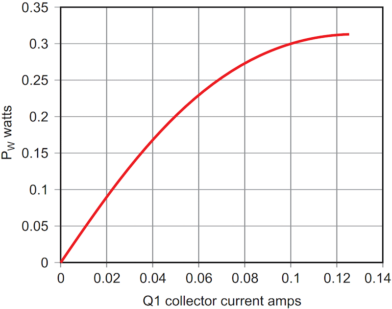
Okay so far. But how does compensation for Figure 1’s nonlinearity happen? Well, happily the function of Q1’s PW vs collector current I isn’t linear either. In fact PW = 5 V·I – I2R3. That quadratic I2 term is the key. It creates the lovely linearizing curve shown in Figure 3.
 |
|
| Figure 3. | This graph details Q1 power dissipation vs collector current. PW = 5 V·I – I2R3. |
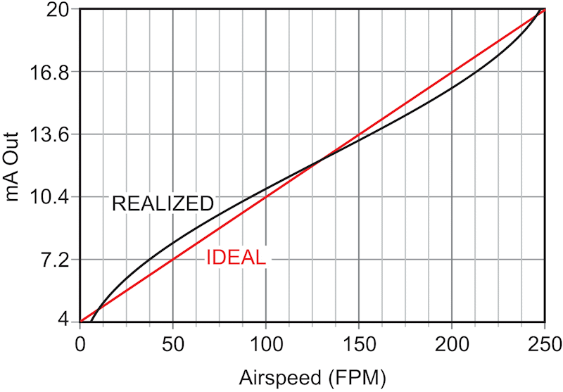
The 2nd-order curvature of Figure 3 compensates for the bend in Figure 1. Although the match isn’t perfect, when converted to the 4-20 mA by opamp A1, the realized output is a calibrated readout of air speed that differs from ideal by less than ±5% from 0 to 250 fpm, as shown in Figure 4.
 |
|
| Figure 4. | This graph’s data relates anemometer output vs airspeed: FPM = 15.6(IOUT – 4 mA) ±10 fpm. |